

The dm package reduces your mental strain when working with many tables. It connects your data, while still keeping them in their original tables. You can easily perform operations on all tables, visualize how they’re connected, and integrate databases.
 Photo by Tobias Fischer
Rather than writing out the relational structure in code while connecting the sources, dm packages them in data. This workflow prevents you from inconsistently updating tables, making copies due to redundancies and, more generally, losing track of decisions made in a data pipeline.
A case study
To demonstrate dm’s benefits, let’s compare some workflows using data from the nycflights13 package.
We want to get the data to analyze arrival delays of flights of planes built more than 30 years ago. For these flights, we also want to check if they departed for destinations in the south. We use methods from the dplyr package, the grammar for data manipulation from the tidyverse.
This requires columns lon (longitude) from table airports, year
from table planes and arr_delay (arrival delay) from flights. We
can do this by performing multiple joins, one after another, as you
might be used to:
library(nycflights13)
library(dplyr)
planes_join <- planes %>%
  rename(production_year_plane = year) %>%
  left_join(flights, by = "tailnum") %>%
  left_join(airports, by = c("dest" = "faa")) %>%
  select(lon, year, production_year_plane, dest)

planes_join %>%
  filter(production_year_plane < 1983)
## # A tibble: 1,432 x 4
##      lon  year production_year_plane dest
##    <dbl> <int>                 <int> <chr>
##  1 -95.3  2013                  1965 IAH
##  2 -95.3  2013                  1965 IAH
##  3 -95.3  2013                  1965 IAH
##  4 -95.3  2013                  1965 IAH
##  5 -87.9  2013                  1959 ORD
##  6 -97.0  2013                  1959 DFW
##  7 -97.0  2013                  1959 DFW
##  8 -97.0  2013                  1959 DFW
##  9 -90.4  2013                  1959 STL
## 10 -97.0  2013                  1959 DFW
## # … with 1,422 more rows
Fair enough, you might say — to keep an overview, we can reduce the 34
columns using select(), then filter(). But what do you do once there
are 30 tables, possibly from databases you’re working with? Is this
still a workable solution? And how sure are we that we truly only need
these three columns?
dm
On your dm object, you can directly
apply operations like filter() to all your tables! How so? Because
relations between the objects are already registered in the
dm object, you don’t need to indicate
them.
Not having to state how tables are connected each time you perform a join may make exploratory work a lot easier:
library(dm)
cdm_nycflights13() %>%
  cdm_filter(planes, year < 1983)
## ── Table source ───────────────────────────────────────────────────────────
## src:  <package: nycflights13>
## ── Data model ─────────────────────────────────────────────────────────────
## Data model object:
##   5 tables:  airlines, airports, flights, planes ...
##   53 columns
##   3 primary keys
##   3 references
## ── Rows ───────────────────────────────────────────────────────────────────
## Total: 27583
## airlines: 4, airports: 3, flights: 1432, planes: 29, weather: 26115
This produces an overview of your data sources — all tables still
separated. Also note: there was no need to rename() the column year,
and all tables stay separate.
What if you still wanted to produce a join and check where those flights departed to? Voilà:
cdm_nycflights13() %>%
  cdm_filter(planes, year < 1983) %>%
  cdm_join_tbl(flights, airports)
## # A tibble: 1,432 x 19
##     year month   day dep_time sched_dep_time dep_delay arr_time
##    <int> <int> <int>    <int>          <int>     <dbl>    <int>
##  1  2013     1     1      839            850       -11     1027
##  2  2013     1     1      858            900        -2     1102
##  3  2013     1     1     1219           1220        -1     1415
##  4  2013     1     1     1317           1325        -8     1454
##  5  2013     1     1     1422           1410        12     1613
##  6  2013     1     1     1806           1810        -4     2002
##  7  2013     1     1     1911           1910         1     2050
##  8  2013     1     1     2030           2045       -15     2150
##  9  2013     1     2      535            540        -5      831
## 10  2013     1     2      945            945         0     1113
## # … with 1,422 more rows, and 12 more variables: sched_arr_time <int>,
## #   arr_delay <dbl>, carrier <chr>, flight <int>, tailnum <chr>,
## #   origin <chr>, dest <chr>, air_time <dbl>, distance <dbl>, hour <dbl>,
## #   minute <dbl>, time_hour <dttm>
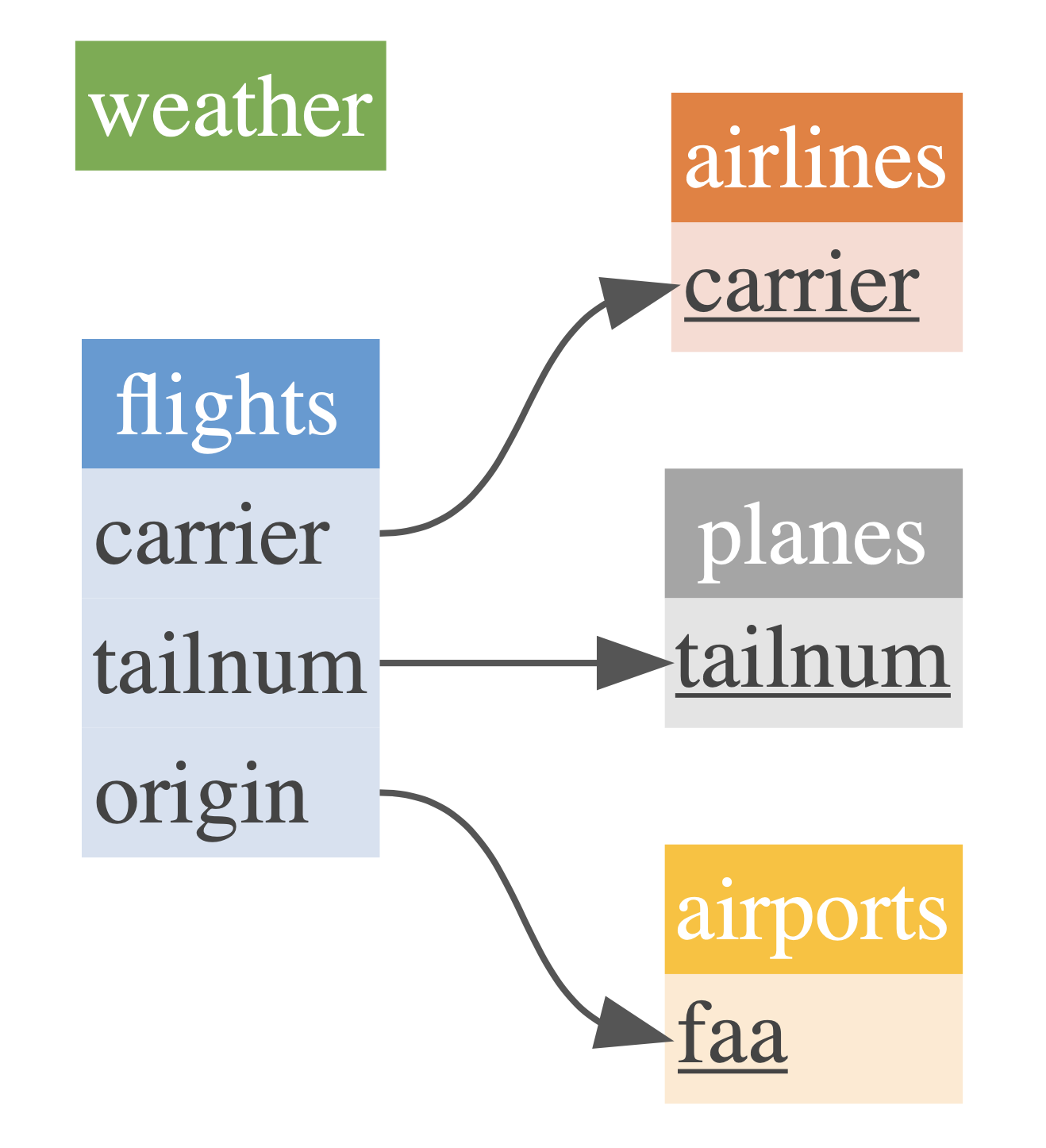
Visualization
You can easily gain a visual overview using cdm_draw(). This results
in pretty, customizable (using cdm_set_colors()) visualizations of how
your data connect.
cdm_nycflights13() %>%
  cdm_set_colors(
    flights = "blue_nb",
    airlines = "orange_nb",
    weather = "green_nb",
    airports = "yellow_nb",
    planes = "light_grey_nb"
  ) %>%
  cdm_draw()
Databases
dm works for both in-memory data and databases. You can easily integrate it into your dbplyr workflow, making for new, powerful ways of analysis.
Feedback
This was just a short glimpse of what dm can do — more posts will follow. Feel free to contribute to this package on Github. Funding for dm is generously provided by Energie360 and cynkra. This package is authored by Tobias Schieferdecker and Kirill Müller.